Multi-fidelity emulation
Use Emukit to build emulators in scenarios where data of different levels of accuracy are available. Use this models in decision loops.
A common issue encountered when applying machine learning to environmental sciences and engineering problems is the difficulty or cost required to obtain sufficient data for building robust models. Possible examples include aerospace and nautical engineering, where it is both infeasible and prohibitively expensive to run a vast number of experiments using the actual vehicle. Even when there is no physical artifact involved, such as in climate modeling, data may still be hard to obtain when these can only be collected by running an expensive computer experiment, where the time required to acquire an individual data sample restricts the volume of data that can later be used for modeling.
Constructing a reliable model when only few observations are available is challenging, which is why it is common practice to develop simulators of the actual system, from which data points can be more easily obtained. In engineering applications, such simulators often take the form of Computational Fluid Dynamics tools which approximate the behaviour of the true artifact for a given design or configuration. However, although it is now possible to obtain more data samples, it is highly unlikely that these simulators model the true system exactly; instead, these are expected to contain some degree of bias and/or noise.
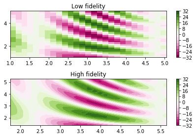
Naively combining observations from multiple information sources could result in the model giving biased predictions which do not accurately reflect the true problem. To this end, multi-fidelity models are designed to augment the limited true observations available with cheaply-obtained approximations in a principled manner. In such models, observations obtained from the true source are referred to as high-fidelity observations, whereas approximations are denoted as being low-fidelity. These low-fidelity observations are then systemically combined with the more accurate (but limited) observations in order to predict the high-fidelity output more effectively.
Emukit offers implementation of a selection Gaussian process multi-fidelity models that can also be combined with other outer-loop applications. To work with an specific example we start loading a problem with two fidelities in which their relationship between is linear. You can check [1] for a graphical representation of this problem. We will use the interval [0,1] as the input domain in our experiment.
from emukit.emukit.test_functions.forrester import forrester, forrester_low

x_train_l = np.atleast_2d(np.random.rand(12)).T
x_train_h = np.atleast_2d(np.random.permutation(x_train_l)[:6])
y_train_l = forrester_low(x_train_l)
y_train_h = forrester(x_train_h)
X_train, Y_train = convert_xy_lists_to_arrays([x_train_l, x_train_h], [y_train_l, y_train_h])
With this code we have just collected some samples in both fidelities and formatted the data in a way that can be understood by Emukit. Emukit expects the final column of the model inputs to contain an index which indicates which fidelity the point belongs to. Normally, high fidelities are more expensive to sample than low fidelities so we have reflected that in the data collection approach.
Now that we have the data, it is time to show how to use Emukit to train a Gaussian process linear multi-fidelity model as proposed in [3]. A non-linear version of this model proposed in [3] is also available. The linear model assumes that the high fidelity is a linear combination of the low fidelity and a delta term that captures the difference between the two. We just need to specify the kernels for the two fidelities and create the model. GPy is used as the modelling framework in this example.
import GPy
from emukit.multi_fidelity.kernels import LinearMultiFidelityKernel
from emukit.multi_fidelity.models import GPyLinearMultiFidelityModel

num_fidelities = 2
kernels = [GPy.kern.RBF(1), GPy.kern.RBF(1)]
linear_mf_kernel = LinearMultiFidelityKernel(kernels)
gpy_linear_mf_model = GPyLinearMultiFidelityModel(X_train, Y_train, linear_mf_kernel, n_fidelities = 2)
We have created the model. The last step is to train it. As the evaluations of the fidelities are exact, we first set the noise parameters to zero by doing
gpy_linear_mf_model.mixed_noise.Gaussian_noise.fix(0)
gpy_linear_mf_model.mixed_noise.Gaussian_noise_1.fix(0)
and complete the training by optimizing the model
gpy_linear_mf_model.optimize()
If you are planning to use the model in a loop (like Bayesian optimization or experimental design) you can load the GPyMultiOutputWrapper in emukit.model_wrappers.gpy_model_wrappers and wrap it.
And that’s it! In the tutorials you can see how to train other available models like the one described in [2], which assumes a non-linear relationship between fidelities.
Check our list of notebooks and examples if you want to learn more about how to do multi-fidelity emulation and other methods with Emukit. You can also check the Emukit documentation.
We’re always open to contributions! Please read our contribution guidelines for more information. We are particularly interested in contributions regarding examples and tutorials.
References on Muti-fidelity emulation
-
[1] Forrester, Alexander I.J., Sóbester, András and Keane, Andy J. (2007) Multi-fidelity optimization via surrogate modelling. Proceedings of the Royal Society of London A, 463 (2088), 3251-3269.
-
[2] Kennedy, M.C. and O’Hagan, A., 2000. Predicting the output from a complex computer code when fast approximations are available. Biometrika, 87(1), pp.1-13.
-
[3] Perdikaris, P., Raissi, M., Damianou, A., Lawrence, N.D. and Karniadakis, G.E., 2017. Nonlinear information fusion algorithms for data-efficient multi-fidelity modelling. Proc. R. Soc. A, 473(2198), p.20160751.
