Bayesian Optimization
Bayesian optimization is a sequential decision making approach to find the optimum of objective functions that are expensive to evaluate.
Bayesian optimization (see [1] for a review) focuses on global optimization problems where the objective is not directly accessible. This can be the case when evaluating the objective comes with a very high cost, e.g. training a large neural network in a large dataset, or because it is embodied in some physical process, e.g. optimizing a synthetic gene to over produce a protein in a cell. Other examples are problems in robotics, inference with intractable likelihoods, compiler optimization, etc.
Given some function defined in a constrained input space, the goal is to find the location of its minimum (or maximum). For illustrative purposes of how to solve these problems with Emukit, we start by loading the Branin function. We define the input space to be .
from emukit.test_functions import branin_function
from emukit.core import ParameterSpace, ContinuousParameter

f, _ = branin_function()
parameter_space = ParameterSpace([ContinuousParameter('x1', -5, 10),
                                  ContinuousParameter('x2', 0, 15)])
In general cases we assume that the function does not have explicit form and that it is expensive to evaluate. This means that to find the optimum we’ll need to run a finite, and typically small, number of evaluations. Selecting these evaluations smartly is the key to approaching the optimum with a minimal cost. This transforms the original optimization problem into a sequence of decision problems (of where to select the best next location). In Bayesian optimization these problems are solved using principles of statistical inference and decision theory.
How is it done? The first step is to build a model for the objective function. This model should capture our prior beliefs about the function and can be either generic or it can encode some prior structural knowledge about the problem. Every time we evaluate the objective the model is updated with the collected data. Following with our example, let’s start by collecting 5 points at random and use them to train a Gaussian process [2] with GPy.
from emukit.experimental_design.model_free.random_design import RandomDesign
from GPy.models import GPRegression
from emukit.model_wrappers import GPyModelWrapper

design = RandomDesign(parameter_space) # Collect random points
num_data_points = 5
X = design.get_samples(num_data_points)
Y = f(X)
model_gpy = GPRegression(X,Y) # Train and wrap the model in Emukit
model_emukit = GPyModelWrapper(model_gpy)
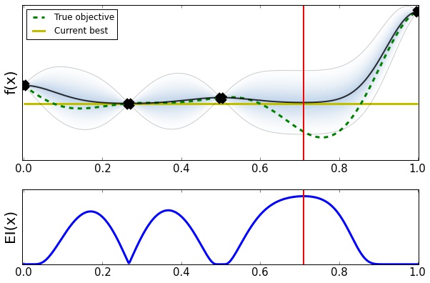
The next step in Bayesian optimization is to define an acquisition function able to quantify the utility of evaluating each point the input domain. The central idea of the acquisition function is to trade off the exploration of regions where the model is uncertain and the exploitation of the model’s confidence about good areas of the input space. There are a variety of acquisition functions in Emukit. In this example the expected improvement [3], that computes in expectation how much we can improve with respect to the current best observed location.
from emukit.bayesian_optimization.acquisitions import ExpectedImprovement

expected_improvement = ExpectedImprovement(model = model_emukit)
Given the model and the acquisition, Bayesian optimization iterates the following three steps until it achieves a predefined stopping criterion (normally using a fixed number of evaluations).
- Find the next point to evaluate the objective by using a numerical solver to optimize the acquisition/utility.
- Evaluate the objective in that location and add the new observation to the data set.
- Update the model using the currently available data.
In Emukit, we first create the Bayesian optimization loop using the previously defined objects.
from emukit.bayesian_optimization.loops import BayesianOptimizationLoop

bayesopt_loop = BayesianOptimizationLoop(model = model_emukit,
                                         space = parameter_space,
                                         acquisition = expected_improvement,
                                         batch_size = 1)
The bach size is set to one in this example as we’ll collect evaluations sequentially but parallel evaluations are allowed. Once the loop is created we run it for some iterations, 30 in our example.
max_iterations = 30
bayesopt_loop.run_loop(f, max_iterations)
And that’s it! You can check the obtained the results looking into the state of the loop or by running:
results = bayesopt_loop.get_results()
Note that you can use other models and acquisitions of your own in this loop.
Check our list of notebooks and examples if you want to learn more about how to do Bayesian optimization and other methods with Emukit. You can also check the Emukit documentation.
We’re always open to contributions! Please read our contribution guidelines for more information. We are particularly interested in contributions regarding examples and tutorials.
References on Bayesian optimization
-
[1] Shahriari, B., Swersky, K., Wang, Z., Adams, R. P, de Freitas, N., (2016). Taking the Human Out of the Loop: A Review of Bayesian Optimization. Proceedings of the IEEE, Vol.104, No.1, January 2016.
-
[2] Rasmussen, C. E. and Williams, C. K. I., (2005). Gaussian Processes for Machine Learning (Adaptive Computation and Machine Learning. The MIT Press, 2005.
-
[3] Jones, D. R., Schonlau, M., Welch, W. J., (1998). Efficient Global Optimization of Expensive Black-Box Functions. Journal of Global Optimization, 1998.